UNIT 5. Regression

6. UNIT 5. Regression#

This Unit includes main introduction to linear and non-linear regression, strongly based in [1].

[1]

Dirk P. Kroese, Zdravko Botev, Thomas Taimre, and Radislav: Vaisman. Data Science and Machine Learning: Mathematical and Statistical Methods. Machine Learning & Pattern Recognition. Chapman & Hall/CRC, 2020. URL: https://acems.org.au/data-science-machine-learning-book-available-download (visited on 2023-08-15).

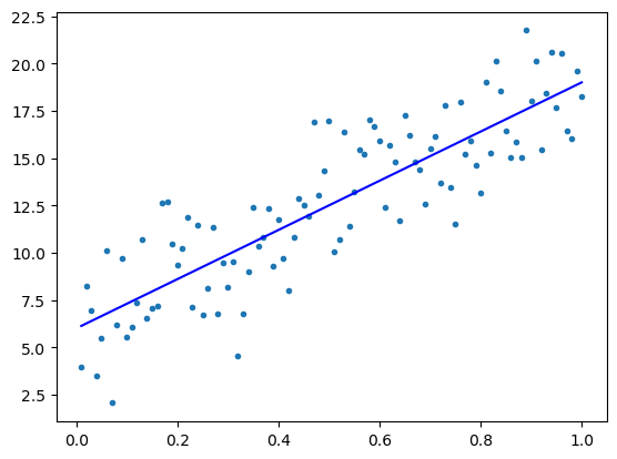
Simple linear regression

""" confpred.py """
import numpy as np
import matplotlib.pyplot as plt
from  numpy.linalg import inv, lstsq, norm
np.random.seed(123)

n = 100
x = np.linspace(0.01,1,100).reshape((n,1))
# parameters
beta = np.array([6,13])
sigma = 2
Xmat = np.hstack((np.ones((n,1)), x)) #design matrix
y = Xmat @ beta + sigma*np.random.randn(n) 

# solve the normal equations
betahat = lstsq(Xmat, y,rcond=None)[0] 

rl = np.zeros(n)  # (true) regression line
u = 0

for i in range(n):
    u = u + 1/n;
    xvec = np.array([1,u])
    rl[i] = xvec.T @ beta;

plt.plot(x,y, '.')
plt.plot(x,rl,'b')
plt.savefig("../figures/linreg.png")

../_images/ee1edb2da17ffa3c4089454ec1929ea8420e5e45eaa398f2c7f9f375dbd0fa1e.png

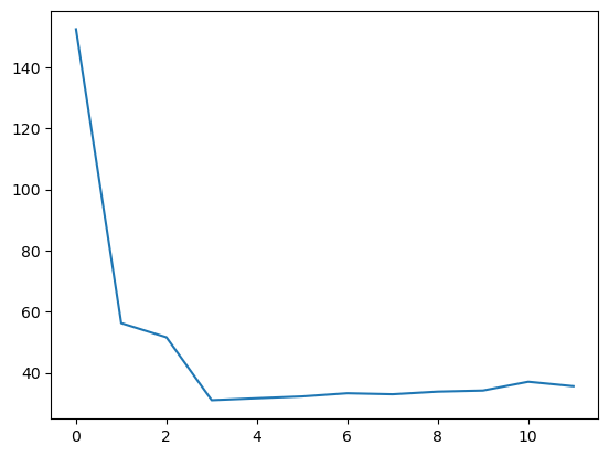
Calculation of the Predicted Residual Sum of Squares (PRESS)

We start by defining that in a multiple linear regression model the response $Y$ depends on a $d$-dimensional explanatory vector $\mathbf{x}=[x_1,\ldots,x_d]^T$ via the relationship: $$Y=\beta_0 + \beta_1 x_1 + \cdots + \beta_d x_d + \varepsilon$$ where $\mathbb{E}\varepsilon=0$ and $\mathbb{Var}\varepsilon =\sigma^2$.

This is true for a given pair $(\mathbf{x},Y)$ of data. If we want to apply it to a whole training set $\mathcal{T}=\{(\mathbf{x_1},Y_1),\ldots,(\mathbf{x_n},Y_n)\}$, we consider a linear model of the form: $$\mathbf{Y}=\mathbf{X}\mathbf{\beta}+\mathbf{\varepsilon}$$

We return here to the polynomial regression problem that we explored in (Chapter 2)[UNIT2-Statistical-Learning.ipynb]. There, we estimated the generalization risk for various polynomial prediction functions using independent validation data. Here we calculate such generalization risk using cross validation and compute the PRESS using $$ \mathrm{PRESS}=\sum_{i=1}^n \left(\frac{e_i}{1-p_i}\right)^2 $$ where $e_i=y_i-\hat{y_i}=y_i-(\mathbf{X}\hat{\mathbf{\beta}})$ is the $i$ th residual and $p_i$ are the diagonal values of the orthogonal projection matrix $\mathbf{X}\mathbf{X}^+$

""" polyregpress.py """
import numpy as np
from numpy.random import rand, randn
from numpy.linalg import norm, solve
import matplotlib.pyplot as plt
from sklearn.preprocessing import PolynomialFeatures

def generate_data(beta , sig, n):
    u = np.random.rand(n, 1)
    y = u ** np.arange(0, 4) @ beta.reshape((4,1)) + sig * np.random.randn(n, 1)
    return u.reshape((n,)), y.reshape((n,))

np.random.seed(12)
beta = np.array([10, -140, 400, -250]);
sig=5; n = 10**2;
u,y = generate_data(beta,sig,n)

K = 12 #maximum number of parameters
press = np.zeros(K)
for k in range(K):
    poly = PolynomialFeatures(k)
    X = poly.fit_transform(u.reshape(-1, 1)) # construct the model matrix
    P = X @ (np.linalg.inv(X.T @ X) @ (X.T)) # hat matrix
    e = y - P @ y

    press[k] = np.mean(np.power(np.divide(e,(1-np.diag(P))),2))

plt.plot(press) 

[<matplotlib.lines.Line2D at 0x11953fd90>]

../_images/ce493329b2255ca7625aca6ceb49aa7ffcf599bfa11d1e4c177fa391134e8da7.png

Inference for Normal Linear Models

Example on the yield of crop for four different crop treatments (columns) on four different plots (rows)

""" crop.py """
import numpy as np
from scipy.stats import f
from numpy.linalg import lstsq, norm 
 
yy = np.array([9.2988, 9.4978, 9.7604, 10.1025,
      8.2111, 8.3387, 8.5018,  8.1942,
      9.0688, 9.1284, 9.3484,  9.5086,
      8.2552, 7.8999, 8.4859,  8.9485]).reshape(4,4).T
print(yy)

[[ 9.2988  8.2111  9.0688  8.2552]
 [ 9.4978  8.3387  9.1284  7.8999]
 [ 9.7604  8.5018  9.3484  8.4859]
 [10.1025  8.1942  9.5086  8.9485]]

nrow, ncol = yy.shape[0], yy.shape[1]
n = nrow * ncol
y = yy.reshape((16,))
X_1 = np.ones((n,1))

KM = np.kron(np.eye(ncol),np.ones((nrow,1)))
KM[:,0]
X_2 = KM[:,1:ncol]
IM = np.eye(nrow)
C = IM[:,1:nrow]

X_3 = np.vstack((C, C))
X_3 = np.vstack((X_3, C))
X_3 = np.vstack((X_3, C))
 
X = np.hstack((X_1,X_2))
X = np.hstack((X,X_3))

print(X)

[[1. 0. 0. 0. 0. 0. 0.]
 [1. 0. 0. 0. 1. 0. 0.]
 [1. 0. 0. 0. 0. 1. 0.]
 [1. 0. 0. 0. 0. 0. 1.]
 [1. 1. 0. 0. 0. 0. 0.]
 [1. 1. 0. 0. 1. 0. 0.]
 [1. 1. 0. 0. 0. 1. 0.]
 [1. 1. 0. 0. 0. 0. 1.]
 [1. 0. 1. 0. 0. 0. 0.]
 [1. 0. 1. 0. 1. 0. 0.]
 [1. 0. 1. 0. 0. 1. 0.]
 [1. 0. 1. 0. 0. 0. 1.]
 [1. 0. 0. 1. 0. 0. 0.]
 [1. 0. 0. 1. 1. 0. 0.]
 [1. 0. 0. 1. 0. 1. 0.]
 [1. 0. 0. 1. 0. 0. 1.]]

p = X.shape[1] #number of parameters in full model
betahat = lstsq(X, y,rcond=None)[0]  #estimate under the full model

ym = X @ betahat

X_12 = np.hstack((X_1, X_2)) #omitting the block effect
k = X_12.shape[1] #number of parameters in reduced model
betahat_12 = lstsq(X_12, y,rcond=None)[0] 
y_12 = X_12 @ betahat_12

T_12=(n-p)/(p-k)*(norm(y-y_12)**2 - 
      norm(y-ym)**2)/norm(y-ym)**2

pval_12 = 1 - f.cdf(T_12,p-k,n-p)

X_13 = np.hstack((X_1, X_3)) #omitting the treatment effect
k = X_13.shape[1] #number of parameters in reduced model
betahat_13 = lstsq(X_13, y,rcond=None)[0]
y_13 = X_13 @ betahat_13
T_13=(n-p)/(p-k)*(norm(y-y_13)**2 - 
      norm(y-ym)**2)/norm(y-ym)**2
pval_13 = 1 - f.cdf(T_13,p-k,n-p)

print(pval_12,pval_13)

2.730857009958232e-05 0.03455786133297134

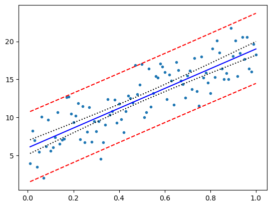
Confidence and prediction intervals

""" confpred.py """
import numpy as np
import matplotlib.pyplot as plt
from scipy.stats import t
from  numpy.linalg import inv, lstsq, norm
np.random.seed(123)

n = 100
x = np.linspace(0.01,1,100).reshape((n,1))
# parameters
beta = np.array([6,13])
sigma = 2
Xmat = np.hstack((np.ones((n,1)), x)) #design matrix
y = Xmat @ beta + sigma*np.random.randn(n) 

# solve the normal equations
betahat = lstsq(Xmat, y,rcond=None)[0] 
# estimate for sigma
sqMSE = norm(y - Xmat @ betahat)/np.sqrt(n-2) 

tquant = t.ppf(0.975,n-2) # 0.975 quantile 
#upper/lower conf. limits
ucl = np.zeros(n)
lcl = np.zeros(n)  
upl = np.zeros(n)  
lpl = np.zeros(n)  
rl = np.zeros(n)  # (true) regression line
u = 0

for i in range(n):
    u = u + 1/n;
    xvec = np.array([1,u])
    sqc = np.sqrt(xvec.T @ inv(Xmat.T @ Xmat) @ xvec)
    sqp = np.sqrt(1 + xvec.T @ inv(Xmat.T @ Xmat) @ xvec)
    rl[i] = xvec.T @ beta;
    ucl[i] = xvec.T @ betahat + tquant*sqMSE*sqc;
    lcl[i] = xvec.T @ betahat - tquant*sqMSE*sqc;  
    upl[i] = xvec.T @ betahat + tquant*sqMSE*sqp;
    lpl[i] = xvec.T @ betahat - tquant*sqMSE*sqp;

plt.plot(x,y, '.')
plt.plot(x,rl,'b')
plt.plot(x,ucl,'k:')
plt.plot(x,lcl,'k:')
plt.plot(x,upl,'r--')
plt.plot(x,lpl,'r--') 

[<matplotlib.lines.Line2D at 0x12935b790>]

../_images/87e7685bf2d1b82c95bd05ca97db0cbb1b4c9946dc17d942ff9ef3a4fc0d4119.png

Linear models with python statsmodels

A simple calculation of the linear model for a bidimensional regression with the ordinary least squares model (ols). Case with two quantitative variables:

""" snippets.py """ 
# %%%%%%%%%%%%%%%%%%%%%%%%%%%%%%%%%%%%%%%%%%%%%%%%%%%%%%%%%%%%%%%%%%%%
import matplotlib.pyplot as plt
import pandas as pd
import statsmodels.api as sm
from statsmodels.formula .api import ols
# %%%%%%%%%%%%%%%%%%%%%%%%%%%%%%%%%%%%%%%%%%%%%%%%%%%%%%%%%%%%%%%%%%%%
myData = pd.DataFrame ({'y' : [10 ,9 ,4 ,2 ,4 ,9] ,
'x1' : [7.4 ,1.2 ,3.1 ,4.8 ,2.8 ,6.5] ,
'x2' : [1 ,1 ,2 ,2 ,3 ,3]})
mod = ols("y~x1+x2", data= myData )
mod_matrix = pd.DataFrame (mod.exog , columns =mod. exog_names )
print ( mod_matrix )

   Intercept   x1   x2
      1.0  7.4  1.0
      1.0  1.2  1.0
      1.0  3.1  2.0
      1.0  4.8  2.0
      1.0  2.8  3.0
      1.0  6.5  3.0

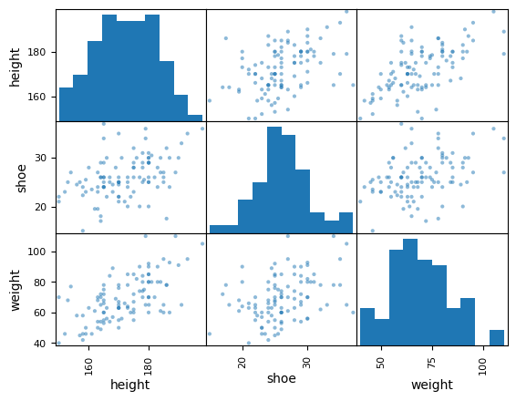
In the second example, we treat the student survey dataset, that contains measurements such as weight, height, sex, etc with $n=100$ university students sample.

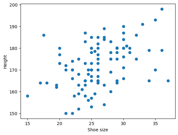
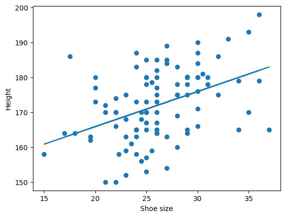
Let us study the relationaship between the shoe size (explanatory variable) and the height (response variable).

# %%%%%%%%%%%%%%%%%%%%%%%%%%%%%%%%%%%%%%%%%%%%%%%%%%%%%%%%%%%%%%%%%%%%
survey = pd.read_csv ('https://raw.githubusercontent.com/DSML-book/Programs/master/Chapter5/survey.csv')
plt.scatter(survey.shoe , survey.height)
plt.xlabel("Shoe size")
plt.ylabel("Height")

Text(0, 0.5, 'Height')

../_images/c34a7aa604e3d50fb387b1bb19d383115aaa32d7914e36ddd266687cca37d376.png

Parameter estimation. Let us find $\beta_0$ and $\beta_1$.

# %%%%%%%%%%%%%%%%%%%%%%%%%%%%%%%%%%%%%%%%%%%%%%%%%%%%%%%%%%%%%%%%%%%%
model = ols("height~shoe", data=survey ) # define the model
fit = model.fit () #fit the model defined above
b0 , b1 = fit.params
print (fit.params )

Intercept    145.777570
shoe           1.004803
dtype: float64

we will now plot the estimated line on the data:

# %%%%%%%%%%%%%%%%%%%%%%%%%%%%%%%%%%%%%%%%%%%%%%%%%%%%%%%%%%%%%%%%%%%%
plt.plot(survey.shoe , b0 + b1* survey.shoe)
plt.scatter(survey.shoe ,survey.height)
plt.xlabel("Shoe size")
plt.ylabel("Height")

Text(0, 0.5, 'Height')

../_images/301d42775332e940dd0eaa5722a0645efe7f57d991384e3e3fa7c7ece122cbd1.png

the summary of the results can be obtained by the summary method:

coef: Estimates of the parameters
std error: standard deviations of the regression line (suare root of the variances)
t: Student’s t-test statistics associated with the hypotheses $H_0:\beta_i=0$ and $H_1:\beta_i\neq 0$, for $i=0,1$
$P>|t|$: P-value of the Student’s test
$[0.025,0.975]$: 95% confidence intervals for the parameters.
R-squared: coefficient of determination $R^2$ (percentage of variation explained by the regression).
F-statistic: $F$ statistic associated with testing the full model against the default model.
AIC: Akaike information criterion

# %%%%%%%%%%%%%%%%%%%%%%%%%%%%%%%%%%%%%%%%%%%%%%%%%%%%%%%%%%%%%%%%%%%%
print (fit.summary ())

                            OLS Regression Results                            
==============================================================================
Dep. Variable:                 height   R-squared:                       0.178
Model:                            OLS   Adj. R-squared:                  0.170
Method:                 Least Squares   F-statistic:                     21.28
Date:                Mon, 06 Nov 2023   Prob (F-statistic):           1.20e-05
Time:                        07:45:24   Log-Likelihood:                -363.88
No. Observations:                 100   AIC:                             731.8
Df Residuals:                      98   BIC:                             737.0
Df Model:                           1                                         
Covariance Type:            nonrobust                                         
==============================================================================
                 coef    std err          t      P>|t|      [0.025      0.975]
------------------------------------------------------------------------------
Intercept    145.7776      5.763     25.296      0.000     134.341     157.214
shoe           1.0048      0.218      4.613      0.000       0.573       1.437
==============================================================================
Omnibus:                        1.958   Durbin-Watson:                   1.772
Prob(Omnibus):                  0.376   Jarque-Bera (JB):                1.459
Skew:                          -0.072   Prob(JB):                        0.482
Kurtosis:                       2.426   Cond. No.                         164.
==============================================================================

Notes:
[1] Standard Errors assume that the covariance matrix of the errors is correctly specified.

Only 17.8% of the height is explained by the shoe size.

If we check the p-value of the slope we see that it is signifficantly different than zero (small p-value).

# %%%%%%%%%%%%%%%%%%%%%%%%%%%%%%%%%%%%%%%%%%%%%%%%%%%%%%%%%%%%%%%%%%%%
dir(fit)
# %%%%%%%%%%%%%%%%%%%%%%%%%%%%%%%%%%%%%%%%%%%%%%%%%%%%%%%%%%%%%%%%%%%%
fit.pvalues[1]

1.1993996732477541e-05

Now we will add additional features (weight): $$height=\beta_0 + \beta_1 shoe + \beta_2 weigth + \varepsilon$$

# %%%%%%%%%%%%%%%%%%%%%%%%%%%%%%%%%%%%%%%%%%%%%%%%%%%%%%%%%%%%%%%%%%%%
model = ols("height~shoe+weight", data=survey)
fit = model.fit ()
axes = pd.plotting.scatter_matrix(survey[['height','shoe','weight']])
plt.show()

../_images/60bd26cd81eb03cc2b4995a06676f9e02ae6ba1d913652facd9786bca91a2069.png

# %%%%%%%%%%%%%%%%%%%%%%%%%%%%%%%%%%%%%%%%%%%%%%%%%%%%%%%%%%%%%%%%%%%%
fit.summary()

OLS Regression Results
Dep. Variable:	height	R-squared:	0.430
Model:	OLS	Adj. R-squared:	0.418
Method:	Least Squares	F-statistic:	36.61
Date:	Mon, 06 Nov 2023	Prob (F-statistic):	1.43e-12
Time:	07:45:25	Log-Likelihood:	-345.58
No. Observations:	100	AIC:	697.2
Df Residuals:	97	BIC:	705.0
Df Model:	2
Covariance Type:	nonrobust

	coef	std err	t	P>\|t\|	[0.025	0.975]
Intercept	132.2677	5.247	25.207	0.000	121.853	142.682
shoe	0.5304	0.196	2.703	0.008	0.141	0.920
weight	0.3744	0.057	6.546	0.000	0.261	0.488

Omnibus:	1.647	Durbin-Watson:	1.824
Prob(Omnibus):	0.439	Jarque-Bera (JB):	1.103
Skew:	-0.133	Prob(JB):	0.576
Kurtosis:	3.440	Cond. No.	508.

Notes:
[1] Standard Errors assume that the covariance matrix of the errors is correctly specified.

The F-statistic is used to test whether the full model (here with two explanatory variables) is better at “explaining” the height than the default model. The P-value obtained says that at least one of the two variables is associated with the height.

# %%%%%%%%%%%%%%%%%%%%%%%%%%%%%%%%%%%%%%%%%%%%%%%%%%%%%%%%%%%%%%%%%%%%
table = sm.stats.anova_lm(fit)
print(table)

            df       sum_sq      mean_sq          F        PR(>F)
shoe       1.0  1840.467359  1840.467359  30.371310  2.938651e-07
weight     1.0  2596.275747  2596.275747  42.843626  2.816065e-09
Residual  97.0  5878.091294    60.598879        NaN           NaN

# %%%%%%%%%%%%%%%%%%%%%%%%%%%%%%%%%%%%%%%%%%%%%%%%%%%%%%%%%%%%%%%%%%%%
model = ols("height~weight+shoe", data=survey)
fit = model.fit ()
table = sm.stats.anova_lm(fit)
print ( table )
# %%%%%%%%%%%%%%%%%%%%%%%%%%%%%%%%%%%%%%%%%%%%%%%%%%%%%%%%%%%%%%%%%%%%
x = {'shoe': [30.0] , 'weight': [75.0]} # new input ( dictionary )
pred = fit.get_prediction(x)
pred. summary_frame(alpha =0.05).unstack ()
# %%%%%%%%%%%%%%%%%%%%%%%%%%%%%%%%%%%%%%%%%%%%%%%%%%%%%%%%%%%%%%%%%%%%
plt.plot(fit.fittedvalues ,fit.resid ,'.')
plt.xlabel ("fitted values")
plt.ylabel ("residuals")

            df       sum_sq      mean_sq          F        PR(>F)
weight     1.0  3993.860167  3993.860167  65.906502  1.503553e-12
shoe       1.0   442.882938   442.882938   7.308434  8.104688e-03
Residual  97.0  5878.091294    60.598879        NaN           NaN

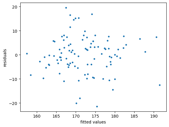
Text(0, 0.5, 'residuals')

../_images/5aed9b7b694f928c8c3082641e3cd438671d3ceaaf876cb86a05f435ae8c3ad6.png

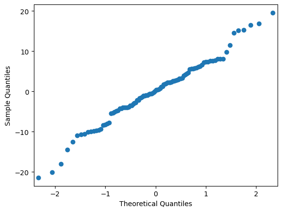
Finallky, we generate a Q-Q plot to explore the normality of the data.

sm.qqplot (fit.resid)
# %%%%%%%%%%%%%%%%%%%%%%%%%%%%%%%%%%%%%%%%%%%%%%%%%%%%%%%%%%%%%%%%%%%%

../_images/45204610989dc2addfd438b27d6fc19cf6a5de606048606d75122197159ae07b.png